Delta Beta instead of Success Rate

Introduction

The success rate is a famous and practical metric used in numerous data science and AI applications and research. Due to its simplicity, Quant researchers also like to use this metric to evaluate their models and strategies as we used it to assess the feasibility of arbitrary return.

However, The success rate has some limitations. One of the important ones is that The success rate does not differentiate between strong and poor returns in positive and negative samples. Consider two data points with +0.1%, +2% returns. success rate counts them as positive samples equally. In addition, The success rate does not consider the market returns and only see trading system result. Therefore, we can not determine the trading system behavior in the volatile or non-volatile market regime. Which means that we need more comprehensive approaches to evaluate trading systems. In this blog, I would like to introduce a metric that we’ve used to measure our model predictive power in different market regimes and benefit from it to optimize our model, i.e. The delta beta. But first, we should know about simple alpha-beta metrics and how we should analyze them.

What is alpha-beta?

Alpha and beta are two well-known metrics for fund managers, portfolio managers, and whoever wants to measure different investment strategies or a portfolio. These metrics represent a portfolio benchmark (a fund benchmark) based on an index. Their formula is:

R = R_f + Beta * ( R_m – R_f ) + Alpha

where

• R represents the portfolio return.
• R_f represents the risk-free rate of return
• R_m represents the index return per a benchmark

If we relax the problem and set R_f to zero, we are going to have

R = beta * R_m + Alpha

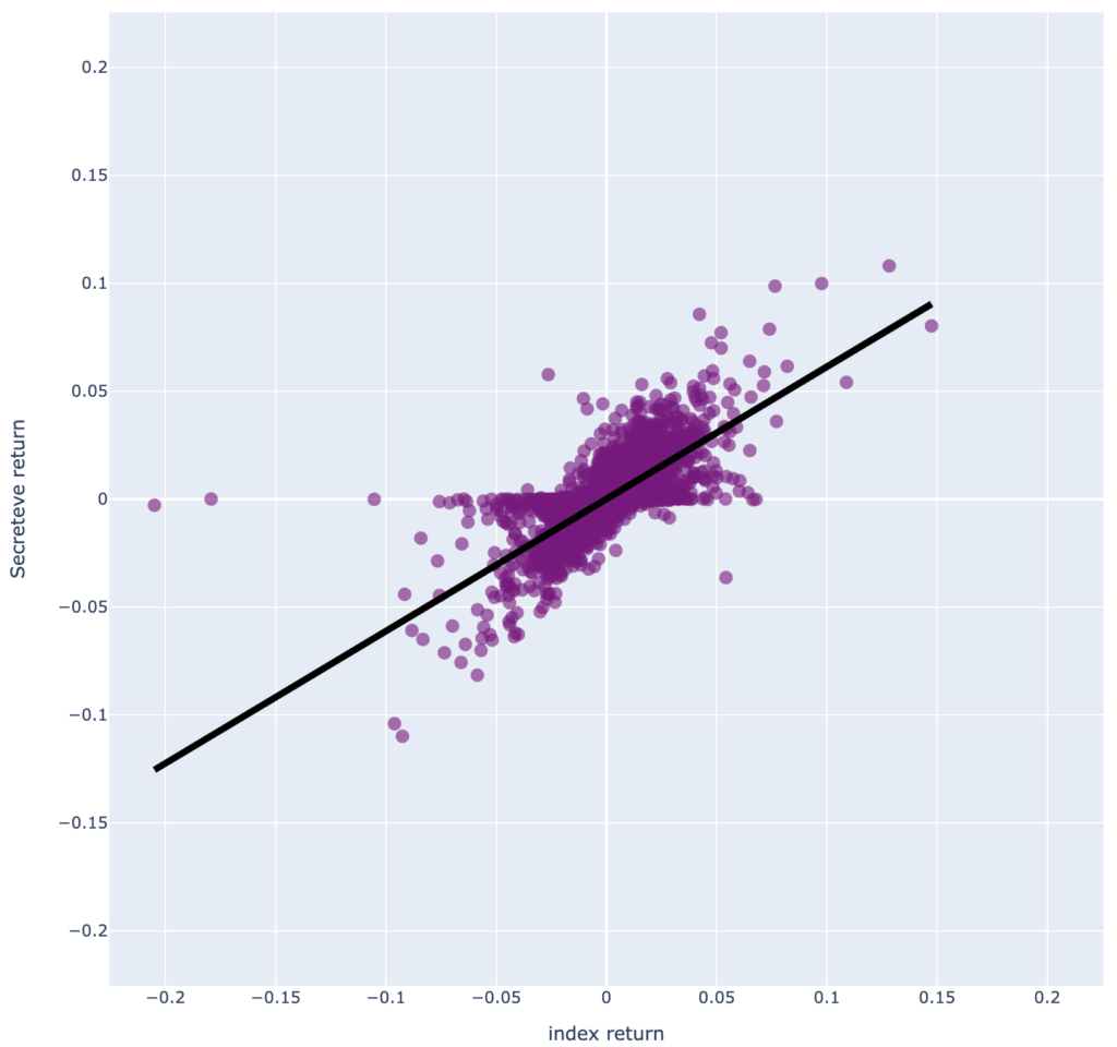
Which is a linear equation. If we collect portfolio returns and corresponding index returns, we can calculate alpha and beta based on their regression formula. There is an example illustrated in Figure 1, where each point is represented by (x= index return, y= portfolio return), and the black line is drawn by the corresponding alpha (y-intercept) and beta (slope) 

Single market Setup

Note that the metrics mentioned above usually measure a portfolio (a group of assets) based on an index. In this article, we want to use a different setup of beta, which can measure a trader and estimate the predictive power of our estimator models. First, let’s assume we want to measure a portfolio that trades one asset.

Two-sided beta

By default, all of the samples participate in alpha and beta calculations. If we separate positive and negative samples, we will have two different sets of alpha and beta representing the risk and performance of the portfolio based on the upside and downside of the index. so we can have beta^positive,beta^negative respectfully as :

R = beta^positive * R_m^positive + Alpha^positive

R = beta^negative * R_m^negative + Alpha^negative

Another critical process that affects trader return is its bet sizing strategy (a strategy that indicates how much should be the size of order). Since here we want to measure the predictive power of the trader/model, I recommend that we test our result with maximum risk. In other words, We can relax our risk management mechanism and only measure predictive power, so the model should create all orders with the entire available portion in a test scenario.

Therefore, We have two lines that calculate trader performance in positive and negative samples independently by the above definitions.

Let’s check beta^positive and beta^negative behavior based on some trader performances.

Scenario 1: suppose a trader has 100 % accuracy in its prediction. Due to our assumption in relaxing the bet sizing mechanism, the trader will have all possible market positive returns in its portfolio benchmark, and its portfolio doesn’t have any negative market return. So the beta^positive is equal to 1, and the beta^negative is equal to 0.

Scenario 2: Suppose that a trader has 0 % accuracy in its prediction. Like scenario 1, we can conclude similarly that the beta^positive is equal to 0, and the beta^negative is equal to 1.

Scenario 3: If a trader has a Buy&Hold strategy, we can say that it has all of the market’s returns, both positive and negative. Therefore, its beta^positive and beta^negative are equal to 1. In the opposite case, If the trader has no trade on the market, it misses all market’s returns, so its beta^positive and beta^negative are 0.

Scenario 4: Suppose that trader has one of these success rates [30%,50%,80%,…], Since we don’t know how good is trader performance in different situations of markets (Is it good in volatile markets? or it’s better in low market returns or vice versa.) Unlike previous scenarios, we can not determine the exact value of either the beta^positive or beta^negative. In this scenario, we should calculate betas directly.

By looking at the results of mentioned scenarios, we can interpret that there is a meaningful relationship in the difference of beta^positive and beta^negative that indicate model performance. From here, In this blog, we refer to this difference as delta beta by the following formulation:

delta beta = beta^positive – beta^negative

Note that the possible outcome for delta beta is in [-1,1], where 1 belongs to the best case (scenario 1), -1 goes to the worse case (scenario 2), and 0 to the balance case (scenario 3) (but there can be other situations that result in balance case, e.x: beta^positive =0.5, beta^negative =0.5 or beta^positive =0.8, beta^negative =0.8).

delta beta as an objective function

We’ve pointed to the weakness of the success rate, the inability to measure model performance in the different market situations, and its inefficiency in being used as an objective function. Also, we introduced the delta beta function to be considered as an alternative measurement metric to evaluate the predictive power of the model/trader. Let’s see how it can happen.

First, let’s define and simulate three different models that have different predictive behavior on various market return values (indication of market volatility)

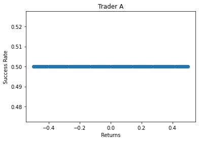
• Trader A: Independent from market return. The chance of success always remains fixed.
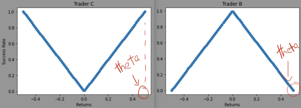
• Trader B: Dependent on market return. It works better on low market returns.
• Trader C: Dependent on market return, It works better on high market returns, Figure 2.

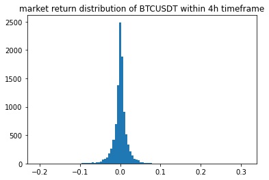
Now Let’s analyze delta beta behavior with some simulations. Note that, In the following experiments, we will sample from the return of the BTCUSDT instrument within a 4h timeframe, Figure 3. We will generate synthetic scenarios by setting different Traders’ parameters and choose random samples from market returns independently.

Independent Case, Trader A.

We are generating experiments with different success rates for trader A, but all of them are independent of the market. Then for each experiment, we’ll calculate delta beta. You can see the linear relation between different success rates and delta beta in Figure 3.

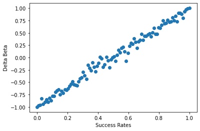
As shown in Figure 3, In the case of independency between model predictive power and market volatility, Delta beta behaves like the Sucess rate; When the Success rate goes higher, Delta Beta also grows and vice versa.

Dependent Cases, Trader B, C.

As we did in the previous case, we will generate numerous independent experiments. Since we want to measure the relation between delta beta and different model behaviors, we need to simulate various model behaviors. to achieve this, we formulate the model success rate as a function of return for both cases with the following equation:

Trader B: success rate = dsr – (dsr/theta)*|market return|

Trader C: success rate = (dsr/theta)*|market return|

Where dsr is the default success rate and theta represents the slope of the relationship. Although we are using a linear relationship here for simplicity, In the real world, it would be a more complex function.

In each experiment, we going to change the theta parameter and fix dsr by a constant value (here we set it up to be 1), which Affects the relationship between model performance and market returns, Figure 5.

Then, we’ll choose many random samples from market returns distribution independently. In each instance, based on the model performance (success rate based on returns, Figure2 ), we’ll decide whether the sample is profitable, loss-making, or negligible to the trader portfolio in experiment simulation. We’ll keep this sampling and simulation till creating a simulated portfolio per experiment. After that, we will calculate the delta beta for each portfolio.

Figures 6 and 7 demonstrate how delta beta could change by different theta values for Trader B, C.

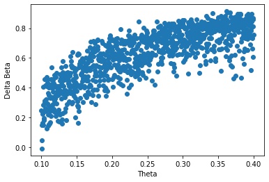
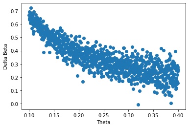
We can easily say that delta beta is sensitive to model predictive power behavior by seeing simulations result. Note that we are not arguing about the feasibility of achieving these results here. It may be impossible to predict the market returns with 100 % accuracy in the real world. Usually, traders’ (models’) behavior is more similar to trader C, where there are trying to react to a volatile situation and significant changes in the market. We simulated both scenarios in extreme cases to emphasize the inability of the success rate to measure the actual models’ behavior. Also, we can see the comparison of delta beta, the success rate, and the beta for those experiments in Figures 8 and 9.

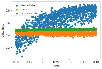
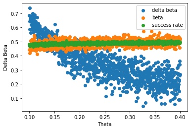
Figures 8 and 9 show that delta beta is sensitive to trader/model behavior (its predictive power dependency on market returns). In contrast, success rate and beta can’t significantly differentiate between models by different behaviors. However, one of the cons of delta beta vs. success rate and beta is its variance. We can address this problem by using classic solutions like measuring samples by the bootstrap approach. Considering the locality principle would be helpful in parameter optimization and measuring model prediction power for different parameters.

It is essential to note that:

• we are trying to evaluate a trader/model predictive power, not a portfolio or fund benchmark. So we are dealing with a single market and the performance of a trader on it.
• Bet sizing strategies are effective on a trader’s performance. But we want to measure the predictive power of the trader. So it is better to assess them independently.

In Conclusion, most traders/models don’t have a uniform behavior for all market returns. Traditional metrics like success rate can’t measure them perfectly. So we’ve tried to use a different setup for well-known metrics, alpha-beta, to measure the predictive power of a model or trader. Quant researchers can use delta beta to measure their developed models or optimize their parameters in their pipelines as we do.

Reza Fahmi, Chief Product Officer, ParticleB